1. Introduction
Carbon dioxide (CO2) forms an essential part of the natural carbon cycle of the Earth, playing a vital role in global warming (Hussain et al., 2024)with the increase in energy demand due to the increase in population and industrialization, the emission of CO2 has increased rapidly in the past few decades. However, the world’s leaders, including the United Nations, are now taking serious action on how to minimize the emission of CO2 into the atmosphere. Towards this end, accurate modeling and monitoring of historical CO2 can help in the development of rational policies. This study aims to analyze the carbon emitted by the Group Twenty (G20. Emissions from industry and fossil fuels reached a record 37.12 billion metric tonnes in 2022. This trend persisted in 2023, with a 1.1% rise in emissions levels, reaching 37.55 billion metric tonnes (International Energy Agency, 2023). Such emissions are a primary factor of climate change, resulting in severe environmental and socio-economic effects like rising global temperature, extreme weather conditions, and biodiversity loss (Intergovernmental Panel on Climate Change, 2023). The main contributors to rising CO2 emissions include fossil fuel use for energy, deforestation, and industrial activities (U.S. Environmental Protection Agency, 2021). Addressing these effects requires adopting eco-friendly energy solutions, boosting energy proficiency, and promoting sustainable land use policies (United Nations, 2021). In 2015, the UN introduced the concept of sustainable development goals with “SDG 13” focusing on the crucial need to address climate change and its impact. All economies worldwide aim to reach carbon neutrality by 2050 through reducing carbon emissions (Dash et al., 2024).
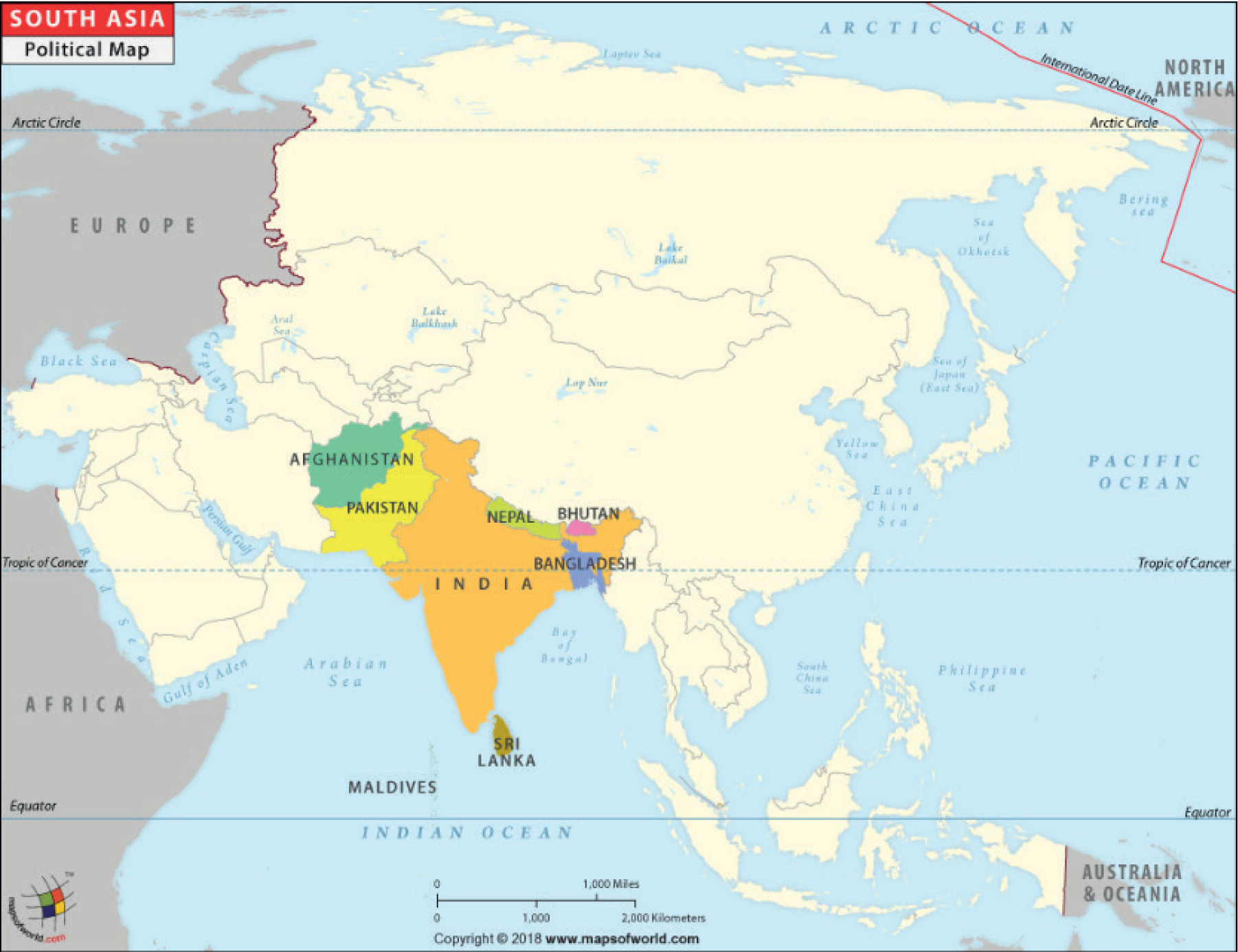
South Asia, an Asian subregion (see Fig. 1), includes the Indus-Ganga plain and peninsular India and encompasses the countries of Afghanistan, Nepal, Bhutan, India, Bangladesh, Sri Lanka, and the Maldives. Having an estimated population of 1.9 billion, the region ranks among the world’s most heavily populated areas. Although South Asia’s per capita GDP is around US$2308, which is significantly lower than lowand middle-income countries’ per capita GDP US $5676 and the world’s, US$13138 (World Bank, 2023). Nonetheless, the region has shown robust growth in recent years. South Asia constitutes one of the regions susceptible to environmental hazards, which requires critical focus. In recent years, the countries in this region have experienced robust economic growth, largely accelerated by industrialization and an expanding financial sector (Rahman et al., 2024). Most of these nations are in a transitional stage characterized by rising industrial activity, urban expansion, and boom consumption due to economic liberalization from the early 1990s. This growth, however, has contributed to an increase in emissions and environmental degradation (Dash et al., 2024).
In 1990, South Asia’s share of global emissions was 3.01%, with individual country contributions of 2.64% from India, 0.27% from Pakistan, 0.05% from Bangladesh, 0.004% from Nepal, 0.009% from Afghanistan, 0.01% from Sri Lanka, 0.004% from the Maldives, and 0.003% from Bhutan. By 2020, this share had increased to 7.50%, with 6.55% from India, 0.54% from Pakistan, 0.25% from Bangladesh, 0.04% from Nepal, 0.02% from Afghanistan, 0.06% from Sri Lanka, 0.004% from the Maldives, and 0.003% from Bhutan (World Bank, 2023). This rise in emissions emphasizes the rising environmental impact of South Asian countries, addressing the need for effective climate interventions.
Fig. 2 illustrates CO2 emission levels within South Asia over the period 1990-2020. India records the highest and fastest-growing emissions, peaking around 2018-2019 before a slight decline.
Figure 2
Trends of log-transformed CO2 emissions (kt) in South Asian countries, 1990-2020
Source: World Bank WDI data (1990-2020).
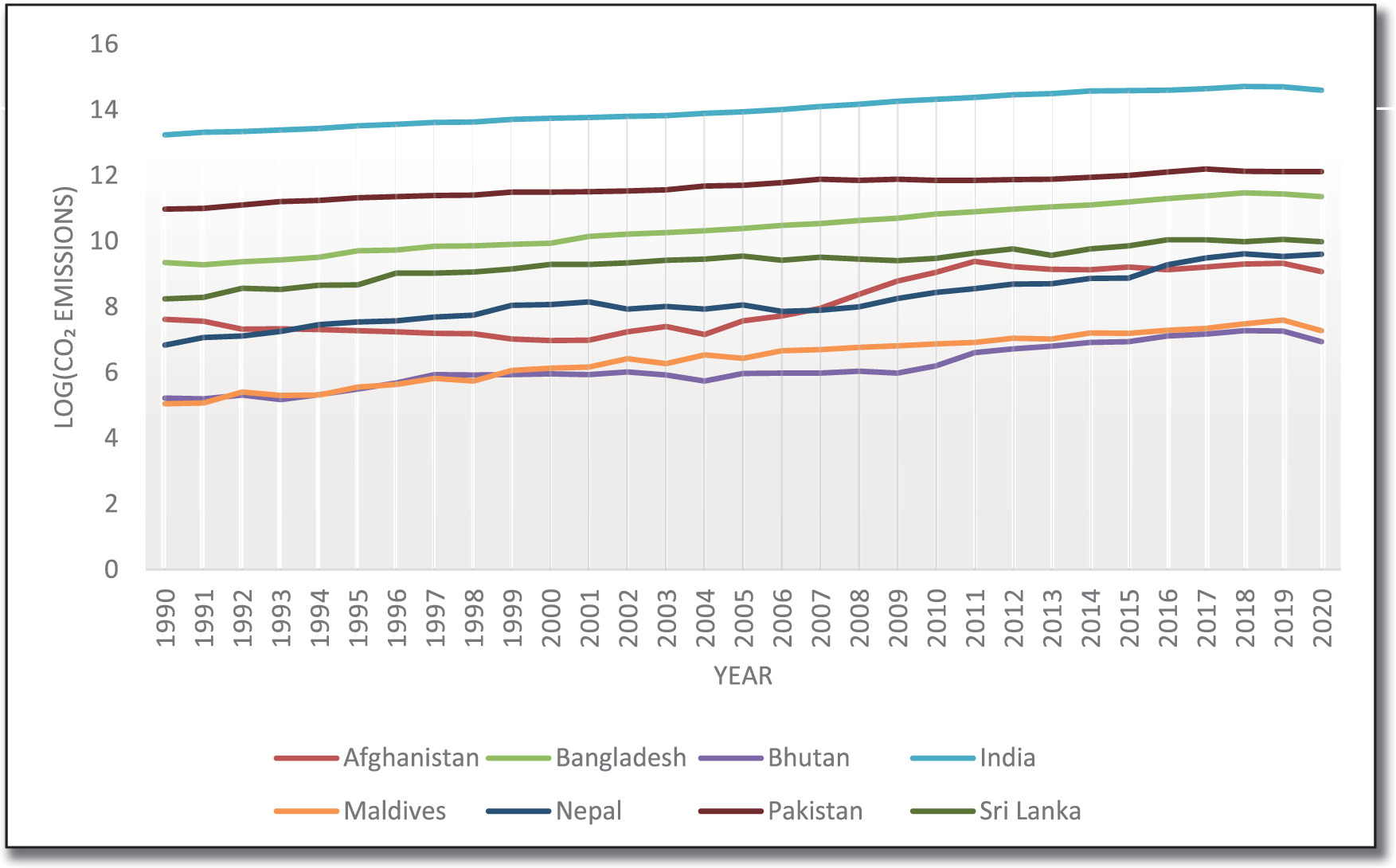
In contrast, other countries like Bangladesh and Pakistan show gradual increases, while Bhutan, the Maldives, and Sri Lanka remain very low contributors. Overall, India’s emissions dominate the regional trend.Economic growth has been strongly associated with higher carbon dioxide (CO2) emissions and energy consumption, which has raised concerns that economic prosperity may have an adverse effect on the environment and climate (González-Álvarez & Montañés, 2023). The level of economic development in any nation depends on various factors. To achieve higher growth, nations adopt different development approaches based on their unique characteristics and the availability of natural resources. However, this growth can adversely affect the environment, including pollution, overuse of resources, and climate change (Aye & Edoja, 2017).
FDI is defined as the process of gaining control over the management and operations of a company in a foreign country or initiating production activities on foreign land. Allowing foreign investment offers several benefits to the host economy, including enhancement of Balance of Payment (BoP), access to advanced technology, employment growth, access to financial resources, and accelerated economic growth (Manocha, 2024)supporting the presence of pollution havens in the region. Long-run results for non-linear FDI depicted positive and significant outcome (using pooled mean group. However, FDI can also have harmful environmental effects, particularly in developing countries, by increasing CO2 emissions.
Population size is directly linked with the CO2 emission, showing a positive relation, indicating that a larger population size leads to higher emissions. This is mainly due to more people requiring greater fossil fuel and natural gas usage, directly affecting the CO2 emission level. Population-driven demand leads to a significant rise in the GDP and national income, which further enhances the energy use and hence CO2 emission (Mohammadi et al., 2020).
In an effort to mitigate the rise in carbon emissions, renewable energy emerges as the most effective solution. Coal, oil, and gas could be replaced with cleaner sources like solar, wind, and hydropower. A plethora of studies support the fact that higher use of renewable energy sources is directly associated with lower greenhouse gas emissions (Mukhtarov et al., 2023; Abubakar et al., 2025). Along with the reduction of greenhouse gas emissions, renewable energy also supports the long-term sustainability and follows the path of green growth and low-carbon development.
Historical evidence shows that industrialization across nations helps to transform their economies towards development. This rapid industrial growth works as a double-edged sword; on one side, it enhances productivity and boosts economic growth, on the other side, it accelerates the CO2 emission and hence significant environmental challenges (Shahbaz et al., 2013). To resolve this paradox, the balance between the growth of the industrial sector along sustainable energy practices is the need of the hour (Acheampong, 2018).
Over the past few decades, these issues have intensified, drawing significant interest from scholars and policymakers. Depth of studies across the world revealed a strong association among energy use, economic growth, FDI, population dynamics, and ecological degradation. But most of the existing literature is centered around the developed economies of the world, such as BRICS, OECD, and ASEAN. It is clearly manifest that the South Asian region is currently among the fastest-growing areas and is extremely vulnerable to the consequences of global climate change. This region is facing the problem of population pressure, rapid urbanization, and industrial expansion, with heavy dependence on fossil fuels, which intensifies the CO2 emissions.
Our study attempts to fill the existing literature gap by considering how CO2 emissions in South Asian countries are influenced by GDP, FDI, POP, REC, and IND over both shorter and longer timeframes. In doing so, it adds to the existing literature while offering new insights into the growth environment relationship in the region. The research is not only of academic interest but also carries practical importance, as it shows how structural factors drive emissions and can guide policymakers toward more effective climate strategies. The findings also help clarify whether FDI in South Asia worsens industrial pollution or instead supports cleaner technologies. Overall, the study sheds light on how economic development interacts with environmental quality, highlighting their trade-offs, and provides useful direction for pursuing sustainable, climate-resilient growth in the region.
In the three main ways this study contributes to the existing literature. First, it provides recent empirical evidence on the determinants of carbon emissions in South Asian countries, a region that has received relatively limited attention in empirical environmental studies. Second, the study applies advanced panel econometric techniques that explicitly account for cross-sectional dependence and heterogeneity across countries, ensuring more reliable long-run and short-run estimates. Third, the findings offer useful policy insights by highlighting the roles of renewable energy consumption, industrialization, and foreign direct investment in shaping environmental outcomes in South Asia.
The paper comprises several structured sections, each dealing with a particular dimension of the topic. Building on the discussion in the previous section, a brief overview of the population growth, FDI, renewable energy consumption, and environmental pollution status of the selected countries will be elaborated in Section 2. The modelling framework and estimation strategy utilized in this study are detailed in Section 3. The result and discussion part of the paper will be highlighted in Section 4. The fifth and final section summarizes the major findings, highlights their relevance for ongoing policy debates, and sets out potential implications for future policy formulation.
1.1 Theoretical background
The empirical framework of this study is grounded in several well-established theoretical perspectives. The relationship between economic growth and environmental degradation is often explained through the Environmental Kuznets Curve (EKC) hypothesis, which suggests a non-linear association between income growth and pollution levels (Leitão, 2024). The role of foreign direct investment is commonly interpreted through the pollution haven and pollution halo hypotheses, which argue that FDI may either increase emissions by relocating polluting industries or reduce emissions through technology transfer and improved efficiency (Benzerrouk et al., 2021). Furthermore, the inclusion of renewable energy consumption is motivated by energy transition theory, which emphasizes the shift from fossil-fuel-based energy systems toward cleaner and more sustainable sources (Yang et al., 2024). Industrialization and population growth are incorporated to capture structural and demographic pressures on environmental quality. Linking these variables to established theories enhances the conceptual clarity of the analysis. These theoretical perspectives jointly inform the selection of variables and the empirical strategy adopted in this study.
2. Review of literature
Recent studies provide evidence of the intricate connections among energy utilization, economic development, and CO2 emissions. Studies employing the Panel ARDL framework in Eastern European and African nations reveal that these variables exhibit strong long-term correlations, underscoring their mutual dependence in shaping environmental outcomes (Meşter et al., 2023; Asongu et al., 2016). A growing strand of literature further confirms that the deployment of renewable energy mainly contributes to emissions reduction. Research on BRICS, ASEAN, and OECD countries demonstrates that renewable energy utilization significantly contributes to lowering CO2 emissions, while simultaneously supporting national sustainability goals and reducing reliance on fossil fuels (Teng et al., 2021; Nordin et al., 2025; Perone, 2024; Sadiq et al., 2024).
The contribution of FDI in influencing emissions has also been widely debated. Research shows that FDI often raises emissions in the short term because it drives industrial activity and energy use. Over time, however, it can also encourage the deployment of cleaner technologies and more sustainable practices, which helps to reduce emissions (Kayani et al., 2023; Teng et al., 2021; Wang & Huang, 2022). Similar dynamics are observed in studies focusing on highly polluted countries and East Asia, where economic growth and trade openness initially amplify emissions but exert limited long-term effects. At the same time, renewable energy adoption does help in curbing emissions, although its impact is often overshadowed by the stronger effects of industrialization and rapid economic expansion (Kayani et al., 2023; Wang & Huang, 2022).
Other dimensions of the growth environment nexus have also been explored. Zaidi and Saidi (2018), analysing Sub-Saharan Africa between 1990 and 2015, found that economic growth enhances health expenditure through its effect on air quality, as shown by the Panel ARDL and VECM Granger causality approaches. Raihan et al. (2024), studying the G-7 economies, observed that the digital economy helps lower emissions in the long run, while urbanization, technological progress, economic growth, and financial accessibility tend to exacerbate them. In the short run, however, both financial accessibility and the digital economy contribute positively by reducing CO2 emissions, whereas economic growth continues to push emissions upward. Similarly, Sadiq et al. (2024), using a CS-ARDL approach for BRICS nations, highlighted the effectiveness of sustainable financing, carbon pricing policies, ecological innovation, and clean energy sources in reducing pollutant emissions. Asumadu-Sarkodie et al. (2017) indicate that industrialization is the foremost contributor to raising emissions, while economic development helps to reduce them. Likewise, Azam et al. (2022), examining six OPEC countries, showed that urbanization, energy use, industrialization, and trade increase emissions, whereas economic growth tends to offset some of these effects.
3. Data Source and Methodology
3.1. Data and Variables
This study examines how the South Asian countries’ carbon emissions were affected between 1990 and 2020 by factors such as LGDP, LFDI, LPOP, LREC, and LIND. Annual data spanning 1990 to 2020 from the World Bank’s World Development Indicators (WDI) are used in the current analysis. The model consists of Carbon dioxide emissions as an endogenous variable that is expressed in kilotons. The LGDP, LFDI, LPOP, LREC, and LIND are the explanatory variables in our research. Table 1 describes the selected variables.
Table 1
Description and Source of Variables
This study examines the long- and short-run effects of LGDP, LFDI, LPOP, LREC, and LIND on LCO2 using a log-linear panel econometric framework. The empirical model is specified as follows:
where denotes the country and denotes time (year). All variables are expressed in their natural logarithmic form to ensure linearity, stabilize variance, and enhance interpretability. The logarithmic variables are defined in Table 1.
3.2. Econometric Framework
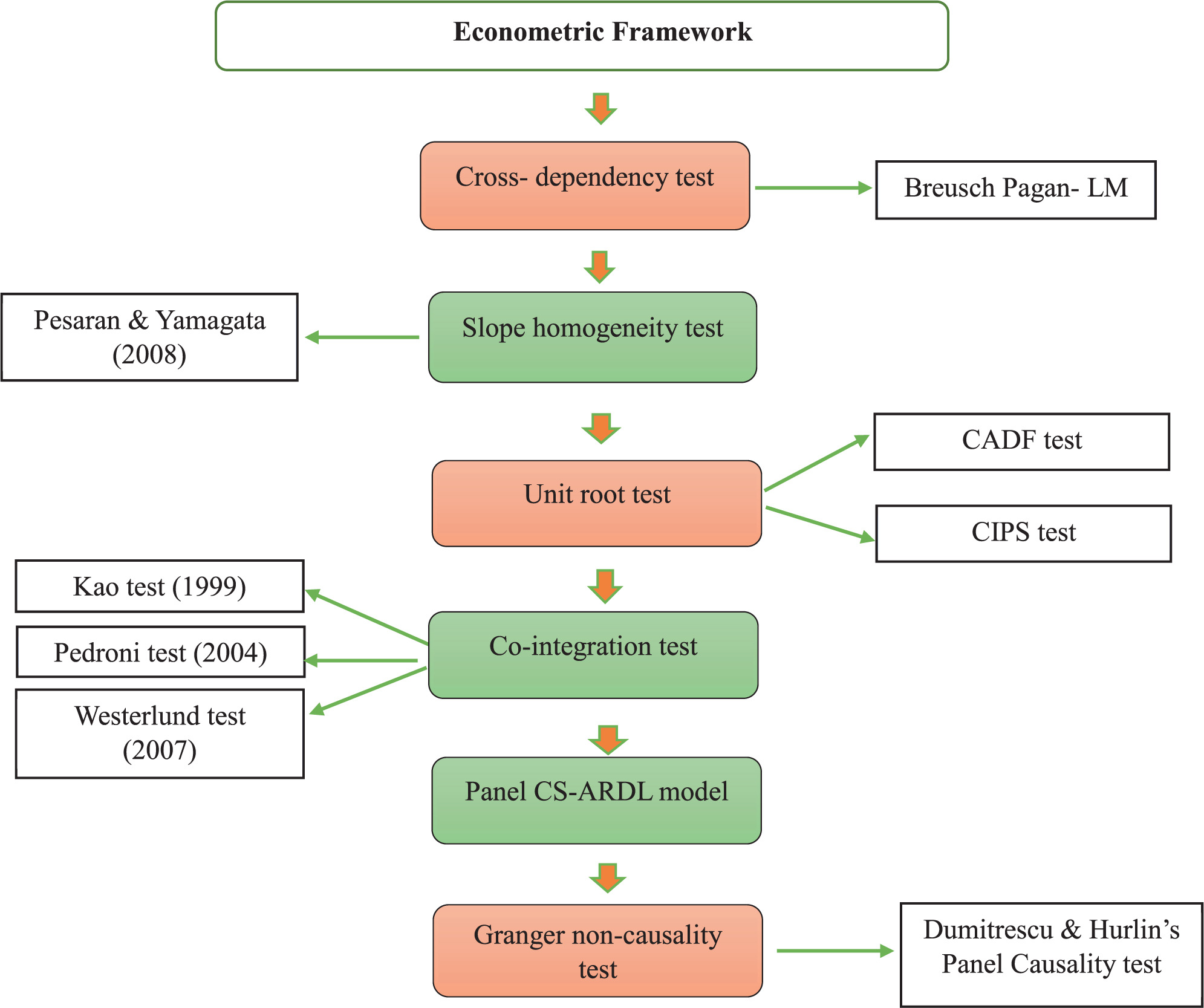
This study employs various panel econometric techniques to evaluate how LGDP, LFDI, LPOP, LREC, and LIND drive LCO2 in South Asia from 1990 to 2020.
3.2.1. Cross-sectional dependency (CD) test
This test is appropriate for panel datasets characterized by a relatively small number of cross-sectional units and a relatively long-time dimension. This condition is satisfied in the present study, which includes 8 cross-sectional entities observed over 31 years (Pesaran, 2021). To examine the presence of cross-sectional dependence, the Breusch–Pagan LM test was employed. The Breusch-Pagan (1980) (Breusch & Pagan, 1980) LM test is written by the following expression:
Where N represents the number of cross-sectional entities, Tkl represents the time observation for the cross-sectional entities, k & l represent unique pairs of cross-sectional entities, with l>k,
3.2.2 Slope homogeneity test
The analysis of panel data often faces the challenge of slope heterogeneity stemming from cross-country variations. This research applies the Pesaran and Yamagata (Pesaran & Yamagata, 2008) slope homogeneity test to account for this issue.
3.2.3 Panel stationarity test
The study employs sophisticated panel stationarity methods, such as, Cross-sectionally Augmented Im, Pesaran, and Shin (CIPS) test and the Cointegrated Augmented Dickey-Fuller (CADF) test, to identify the presence of unit roots and determine whether the variables are stationary (Pesaran, 2007). The CADF equation for testing a unit root is expressed as follows:
Where,
The CIPS equation is expressed as follows:
The CIPS statistic is calculated as the average of CADF statistics across entities (Elhaj et al., 2024):
3.2.4 Panel co-integration test
To examine whether the variables in our panel share a long-run relationship, our analysis incorporates three well-established panel cointegration tests, such as Kao (1999) (Kao, 1999)because the null distribution of residual-based cointegration tests depends on the asymptotics of LSDV estimator. In the second half of the paper I study residual-based tests for cointegration regression in panel data. I study Dickey-Fuller (DF, Pedroni (2004) (Pedroni, 2004), and Westerlund (2007) (Westerlund, 2007). Kao and Pedroni tests are both residual-based tests, in which cointegration is confirmed by checking that the error terms of the long-run regression specified are stationary. The main assumption of the Kao test is homogeneity across cross-sectional entities. On the other hand, the Pedroni test allows for heterogeneity across cross-sectional entities. This assumption of the Pedroni test makes it more useful for addressing country-specific dynamics. While Kao and Pedroni tests rely on residuals, the Westerlund approach determines whether cointegration is absent by investigating the presence of error-correction processes. Another more important benefit of this test as it considers the cross-sectional dependency by utilizing the bootstrap method.
3.2.5 Panel CS-ARDL model
Our study uses the Panel Cross-Sectionally Augmented (CS) ARDL model to inquire about the relationship of LGDP, LFDI, LPOP, LREC, and LIND with LCO2. The traditional panel data methods, such as Panel ARDL, FMOLS, and DOLS, are mainly utilized for getting long-run dynamics, but these methods are not appropriate in cases when there is a problem of cross-sectional dependency among cross-sectional entities (Lee et al., 2023). With the aim of solving these problems, we adopted the CS-ARDL model, as formulated by Chudik and Pesaran (Chudik & Pesaran, 2015). This model is more convenient, because it not only provides the long- and short-term dynamics, but also adjusts the existence of unmeasured common components that may lead to CD.
The CS-ARDL model can be written as:
Where, refers to the amount of carbon dioxide emitted by country i during time t; the first summation term denotes the lagged values of LCO2, capturing dynamic persistence; the second summation reflects the long-run impact of the explanatory variable xit=(LGDPit,LFDIit,LPOPit,LRECit,LINDit), and the third summation zt=(ΔLCO2t,ΔLXt) with captures the short-run dynamics. Finally, uit is the error term accounting for unobserved factors.
3.3.6 Causality test
Lastly, to identify the directional influence of one variable on another, the Dumitrescu and Hurlin (Dumitrescu & Hurlin, 2012) panel causality test has been carried out (Elhaj et al., 2024). This test is reliable because it presents compatible results even with CD across units without imposing constraints on the panel data size or structure (whether short or large panels). It utilizes the following equation:
Where, zit and yjt denotes variables of country i at time t. p represents the lag order, assumed to be identical across countries. Parameters Υi and βi vary across groups. Here, the null hypothesis posits no causality from Y to Z, while the alternative implies the presence of causality from Y to Z.
3.2.7 Robustness check
The AMG model is applied to ensure the reliability of the findings. This method, developed by Eberhardt (Eberhardt & Bond, 2009)parameter heterogeneity and cross-section dependence on estimation and inference in macro panel data. We compare the performance of standard panel estimators with that of our own two-step method (the AMG, accounts for CD, non-stationarity, slope heterogeneity, and endogeneity, thereby producing unbiased estimates. This technique is used to address cross-sectional dependence, so its complementarity with the CS-ARDL model allows for generating compatible results. The (Mata et al., 2024). The AMG specification for this study can be expressed as:
Where denotes period dummies in first differences that capture the unobserved common dynamic process, and represents the associated time dummy coefficients. Replacing with the common dynamic factor , the model can be rewritten as:
Finally, the common dynamic effect is extracted as
Following the AMG framework, the variables are initially transformed with group-specific coefficients
4. Results and Discussion
4.1 Results
4.1.1 Summary statistics
Table 2 summarizes the descriptive statistics for the variables taken in this study, highlighting their mean values, variability, and distribution patterns. The majority of indicators show little difference between mean and median values, suggesting balanced distributions. CO2 emissions and FDI show higher variability, while IND is relatively stable. Skewness values indicate both positive and negative asymme-tries, and kurtosis values above three for FDI, POP, and REC reflect the presence of extreme yet meaningful economic variations. The minimum and maximum values reveal substantial ranges, particularly for FDI and POP, indicating significant disparities among observations. Additionally, the standard deviations suggest that REC exhibits moderate dispersion relative to its mean, highlighting variability in REC throughout the dataset.
Table 2
Descriptive Statistics of the Study Variables
4.1.2 Cross-sectional dependency
Table 3 revealed the CD test results, with a significant test statistic of 239.581. These results indicate the rejection of H0 that variables are independent across various cross-sections and confirm the existence of CD between units. This authorizes the presence of interconnections between the units, suggesting that shocks in one cross-sectional unit can affect others. The test indicates that variables across the South Asian countries are interconnected rather than independent. To ensure accurate and robust results, it’s essential to address CD by employing second-generation panel data methods.
4.1.3 Slope homogeneity test
Findings of the slope homogeneity test can be seen in Table 4. The delta statistics are found to be statistically meaningful at the 1% level, thereby rejecting the null hypothesis of identical regression coefficients. Therefore, the influence of regressor variables on the endogenous variable varies across all units. Consequently, the contribution of the regressor variables to the endogenous variable differs across all units. These findings highlight the importance of using estimation methods that account for such heterogeneity to obtain reliable results.
4.1.4 Panel stationarity test
The CADF and CIPS test results are shown in Table 5. At the level form, most variables are identified as non-stationary, with the exclusion of LFDI, which is stationary at the 1% level. Applying the lagged difference shows that all variables reach stationarity at the 1% significance level according to both tests. This indicates that LCO2, LGDP, LPOP, LREC, and LIND are integrated of order one, I(1), while LFDI is integrated of order zero, I(0).
Table 5
Cross-Sectionally Augmented Panel Unit Root Test Results (CADF and CIPS)
The panel stationarity tests results indicate that all variables attain stationarity, either at their levels or following first differencing, indicating the nonexistence of a unit root issue in the dataset considered. This evidence confirms that the majority of attributes require differencing to achieve stationarity, ensuring their suitability for further econometric analysis.
4.1.5 Multicollinearity test
As illustrated in Table 6, the Variance Inflation Factor (VIF) analysis confirms that none of the variables exceed the accepted limit of 10, indicating low multicollinearity, with REC recording the highest at 3.94. The mean VIF of 2.37 further confirms the absence of severe multicollinearity between the explana-tory variables. Hence, the dataset is suitable for regression analysis without concerns of inflated variance due to collinearity.
4.1.6 Cointegration test
The cointegration techniques for panel data proposed by Kao, Pedroni, and Westerlund are implemented to evaluate the long-run association across the variables. The Kao test results confirm cointegration under multiple statistics, with significance at conventional significance levels (1%, 5%, and 10%). Similarly, the Pedroni test provides additional support, as the modified Phillips-Perron statistic is strongly significant, indicating that the variables move collectively over the extended period. The Westerlund variance ratio test is also statistically meaningful at the 10% level, verifying the demonstration of cointegration. Taken together, these findings suggest a persistent long-term equilibrium association among LCO2, LGDP, LFDI, LPOP, LREC, and LIND, thereby justifying the use of long-run estimation techniques in the subsequent analysis. This consistency across different panel cointegration approaches strengthens the reliability of the empirical results. It also indicates that short-term oscillations are unlikely to disrupt the underlying long-term associations among these variables.
Table 7
Panel Cointegration Test Results (Kao, Pedroni, and Westerlund Tests)
4.1.7 Panel CS-ARDL test
The findings from the CS-ARDL model (Table 8) reveal significant insights into the dynamic linkages of LCO2 with its major determinants over the long- and short-run. Over the short run, LREC is significantly associated with lower LCO2, indicating that emissions are reduced by approximately 1.75% for every 1% increase in LREC. This finding indicates that renewable energy adoption directly contributes to reducing environmental degradation. Similarly, LIND displays a significant and positive effect, with LCO2 increasing by 0.15% for every 1% growth in industrial activity, highlighting the environmental costs of expanding industrial output. LFDI demonstrates a modest but statistically significant positive influence in the short run, implying that while investment inflows benefit economic growth, they are also associated with increased environmental pressure. In contrast, LGDP and LPOP do not exhibit significant effects on emissions in the short run, suggesting that their influence materializes more strongly in the long term.
Table 8
CS-ARDL Estimation Results for CO2 Emissions Determinants (1990-2020)
In the long run, the results reinforce the short-run findings while also providing additional evidence of structural relationships. Renewable energy consumption remains highly negative and significant, reflected by a coefficient value of -2.08, confirming its critical contribution in reducing emissions over time. This emphasizes that sustained adoption of renewable energy technologies contributes to long-term environmental sustainability. LIND continues to exert a significant positive association in the long run, with a 0.19 coefficient value, suggesting that while industrial growth boosts economic activity, it simultaneously intensifies ecological stress unless accompanied by cleaner production technologies. Similarly, LFDI is positively and significantly associated with LCO2, though its effect size (0.021) is smaller, indicating that foreign investment is often directed toward energy-intensive and polluting industries. By contrast, LGDP and population again show insignificant coefficients, implying that their direct long-term contribution to emissions is weak compared to structural drivers such as energy use, industrialization, and capital flows.
Taken together, the findings of the CS-ARDL model highlight a clear trade-off among economic drivers and environmental sustainability across the panel. While LREC emerges as a strong mitigating factor for emissions for both immediate and extended periods, industrialization and LFDI act as significant contributors to rising emissions.
4.1.8 Causality test
Insights from the causality assessment, summarized in Table 9, highlight the causal interactions over time between LCO2 and their major determinants. The findings reveal a reciprocal causal association between LGDP and LCO2, with coefficients significant at the 1% level. This signifies that not only does LGDP per capita influence LCO2, but LCO2 also influences the LGDP per capita of the South Asian countries. Similarly, reciprocal causal association exists between LREC and LCO2 and between LIND and LCO2. On the other side, there is a one-way causal association directed from LPOP to LCO2, which signifies that LPOP influences emissions, but LCO2 does not influence LPOP in the study area. Furthermore, there is a one-way causal association directed from LCO2 to LFDI inflows, but not vice versa. Overall, the findings confirmed that economic activity, industrialization, and renewable energy are closely linked to LCO2 dynamics in the panel.
Table 9
Dumitrescu & Hurlin (2012) Granger non-causality test results
4.1.9 Robustness checks
The AMG technique is applied in this research to validate the reliability of the CS-ARDL model findings. The AMG results, presented in Table 10, indicate that LFDI significantly increases LCO2 in the study area. The impact of LREC also confirms that it helps in reducing LCO2. On the other side, LGDP, LPOP, and LIND do not significantly influence emissions. The majority of outcomes remain compatible with those obtained from the CS-ARDL approach, as LREC helps reduce LCO2 while LFDI increases emissions across the panel.
4.2 Discussion
The research seeks to explore how LGDP, LFDI, LPOP, LREC, and LIND influence LCO2 in South Asia over the period 1990-2020.
One of the key findings from the CS-ARDL model indicates that renewable energy consumption (LREC) significantly reduces CO2 emissions (LCO2). This result is consistent with earlier studies (Mehmood et al., 2022; Yang & Umar, 2022; Zardoub, 2024; Hung, 2024; Asongu et al., 2025), which suggest that energy generated from renewable sources such as solar, wind, and hydropower is considerably less harmful to the environment than fossil fuel-based energy. Apart from eliminating carbon emissions, the plunge into green-energy sources also fosters the advancement of diverse emerging technologies (Nepal et al., 2024; Mata et al., 2024).
Population growth is negatively related to LCO2 with no statistical significance, thus being compatible with earlier insights of Al-shammari et al. (2022), who argue that more significant populations do not necessarily imply higher emissions. One of the reasons for these results could be an increase in general reforms and awareness of climate change, which has led to a decrease in individual LCO2, which was lowered as one of their results. In a typical scenario regarding people from developing countries, they still commonly use traditional fuels instead of abandoning fossil fuel use on a larger scale.
On the other side, LFDI significantly increases carbon emissions, compatible with the previous research insights of Shaikh et al. (2024) and Raza et al. (2025). According to Shaikh et al. (2024), LFDI is often directed toward energy-intensive sectors like manufacturing and infrastructure. Although these investments boost economic growth, they also increase fossil fuel consumption.
One of the significant determinants of the increase in CO2 emissions is industrialization, which is compatible with the research findings of (Asumadu-Sarkodie et al., 2017; Azam et al., 2022; Salan et al., 2025). Essentially, industries tend to meet their energy needs through fossil fuel consumption, which is highly carbon-intensive.
The results show that LGDP and LPOP do not have a statistically significant impact on LCO2 in South Asia. This finding suggests that increases in LGDP and LPOP alone do not automatically lead to higher emission levels in the region. One possible explanation lies in the structural characteristics of South Asian economies, where economic growth is increasingly driven by service-oriented activities that are relatively less energy-intensive. In addition, despite rapid population growth, per capita energy consumption in many South Asian countries remains low, which limits the overall impact of population growth on carbon emissions. Furthermore, the regional energy mix continues to be dominated by conventional energy sources, while improvements in energy efficiency and cleaner production technologies remain gradual. As a result, factors such as industrialization patterns and renewable energy adoption play a more decisive role in shaping emission outcomes than income and population growth alone.
The causality results are essential in understanding the association between these variables. Findings revealed that the linkage between LGDP and carbon dioxide levels is two-way, as through a rise in LGDP, emissions to the atmosphere will also go up; at the same time, rising carbon emissions give rise to economic growth as well. These findings are compatible with the previous findings (Dogan et al., 2017; Habimana Simbi et al., 2025; Oprea et al., 2024).
Reciprocal causal association between LREC and LCO2 is found in this study, compatible with the results of (Dogan & Seker, 2016; Habimana Simbi et al., 2025; Wang et al., 2025). A bi-directional causal association was also found between industrialization and LCO2. As industries grow, they increase pollution, but over time, the resulting environmental pressures can slow down further industrial expansion. These findings are compatible with the findings of (Idowu et al., 2023; Yang et al., 2022).
On the other side, LPOP has been connected to emissions as a one-way relationship, compatible with the findings of (Alagirisamy & Manigandan, 2021). Which means that the dynamics of population characteristics influence emissions, but the reverse is not true. Besides that, the study results indicated that carbon dioxide emissions lead FDI inflows; however, there is no causal association directed from LFDI to emissions (Pata et al., 2023). Thus, the clean environment may turn out to be an attraction for investment from overseas.
In summary, these findings highlight that renewable energy, industrialization, and economic activity are major drivers of emission trends in developing economies. They also highlight the importance of policies that carefully balance economic growth with environmental sustainability, ensuring that development strategies are aligned with a clean energy transition.
5. Conclusion and Policy Implications
This study has explored the interconnected dynamics between economic growth, inflow of FDI, population growth, energy from renewable sources, and industrialization in influencing CO2 emissions in South Asian countries. Our analysis indicates that structural elements, such as industrialization and FDI, contribute more significantly to emissions than general economic or population growth. The industrial activities remain the main contributor to rising emissions because they mainly rely on fossil fuels and resource-intensive production procedures. In the same way, although FDI is good for the local economic growth and for bringing in new technologies, most of it is attracted to the power sector, which is the foremost cause of environmental deterioration both in the short and long term. However, renewable energy consumption (REC) remains very capable of dropping carbon emissions. Results confirm that the expansion of green energy use plays a critical role in reducing carbon emissions, with statistically significant impacts manifest in both the long- and short-term. On the other side, economic growth and population were found to have statistically insignificant effects on emissions. These factors are likely to influence energy use and thus emissions, depending on the type of energy and industrial structures that are in place. Therefore, these results together reflect the dual reality facing South Asia: on the one hand, its economic progress has created growth and opportunities, while on the other, it has also increased ecological pressures. Consequently, the main conclusion is that the region’s growth trajectory will not be sustainable if a clean energy revolution, responsible industrial activities, and climate-friendly investment strategies are not prioritized. South Asia is a place where the decision between growth and sustainability can no longer be seen as two separate choices but as a single framework capable of ensuring both well-being and environmental resilience.
The findings of this study highlight critical priorities for decision makers in the South Asian region. Shifting from polluting energy sources to renewable energy resources is more important to prevent environmental degradation. The easiest and fastest way to achieve this is to use solar, wind, hydro, and other green technologies, and for this, the government also needs to provide various incentives like subsidies, tax exemptions, etc. Foreign investment needs to be diverted towards green and sustainable businesses. This process requires not only clean environmental regulation but also several attractive incentives, such as technology sharing and sustainability-related financing. In addition, industrial development should be directed towards cleaner production, with government support in areas such as energy efficiency, eco-innovation, and the circular economy. The growing population and its rapid urbanization cannot be ignored; therefore, proper planning must be done to expand public transport, build community green energy projects, and promote eco-friendly housing. This will ensure that CO2 emissions do not automatically increase due to the naturally increasing demand for transport, energy, and housing. Most importantly, climate measures must be built into economic and industrial policies from the start, rather than viewed in isolation. By integrating development strategies with sustainability goals, South Asia can achieve inclusive prosperity while protecting its environment for the future. In the short run, policies aimed at improving energy efficiency, strengthening environmental regulations, and promoting cleaner production technologies can help mitigate emissions. In the long run, a gradual transition toward renewable energy sources, green industrial policies, and environmentally responsible foreign investment is essential for achieving sustainable growth in South Asia.