1. Introduction
The institutional capital movements, market fluctuations, and liquidity levels are some of the complex interplays that have a deep impact on the developing financial markets, especially in India. Institutional capital movements refer to investments undertaken by major players such as mutual funds, hedge funds, pension funds, and insurance firms. Large-scale investments by these institutions have the potential to significantly influence market pricing and volatility. Inflows and outflows of their investments cause sharp market movements affecting investor sentiment as well as market stability. In this regard, flows of both FIIs and DIIs must be understood as these flows directly impact the functioning of the markets. FIIs are foreign institutions that invest in Indian financial assets and, being foreign, carry foreign capital with them. At the same time, they have a sensitivity toward global economic developments and risk appetites. DIIs, in contrast, are domestic investment and are driven by factors such as domestic economic and regulatory policies. The interplay between these two types of investors significantly contributes to market dynamics. Market volatility measures the rate at which prices move up and down over time; it represents how uncertain and risky the market.
High volatility is associated with a fast pace and directionless change in prices. Low volatility relates to a slow and relatively stable price movement. India VIX is a significant volatility index in the Indian financial space. Since it is derived from the pricing of options on the Nifty 50 index, India VIX represents an advance predictive estimate of expected market volatility. High India VIX is associated with high expected price fluctuations and high market risk, generally prompting investors to be more conservative. In contrast, relatively low India VIX is associated with a relatively stable market context. Institutional flows and market volatility are related and interactive. Large institutional trades may spark volatility, especially in stressed or uncertain markets. On the other hand, increased levels of volatility can scare away institutional investors, forcing capital to withdraw from the market and increasing volatility. Liquidity-the ability to buy or sell an asset with minimal impact on its price-is necessary to ensure markets remain efficient and stable. High liquidity facilitates fast and efficient trades with very minimal price impacts, hence fostering the smooth operation of markets.
On the other hand, reduced liquidity can hinder trading as this leads to a wider bid-ask spread and increased transaction costs. In illiquid markets, even small trades can cause drastic price movements that enhance volatility. Another interesting feature is the liquidity-institutional investment flow relationship. Institutional investors usually require a high level of liquidity to conduct large trades without significant price slippage. In addition, the institutional investment decision depends on the market liquidity level. More importantly, the institutional trading activity can influence the market liquidity as well. Massive selling by institutions drains the market’s liquidity and leaves it scarce for other participants to liquidate their positions. It also forces market declines. The base of the dynamic understanding of the Indian financial market is built on the understanding of the interaction between these three elements: institutional flows, market volatility, and liquidity. This interaction among the components necessitates an integral view of the market analysis based on the total impact of all these elements.
For policymakers and regulators, an understanding of such associations is indispensable for effective policies to promote stability in the market, improve efficiency in the market, and attract institutional investment. Policymakers are thus able to promote a more favorable environment for sustained economic growth and development through the observation of institutional flows, assessment of market volatility via the India VIX, and ensuring adequate market liquidity. Investors will find that this is the best way to make informed investment decisions and effectively manage risk, given the interaction among these elements in more accurately evaluating market conditions, foreseeing possible risks, and improving their investment strategies. The paper contributes by jointly analyzing institutional flows, volatility, and liquidity in a post-COVID setting with the help of GARCH and VAR models. The integrated approach and recent dataset (2018-2024) make this different from earlier studies analyzing these relationships.
1.1 Literature review
The literature on the dynamics of financial markets, specifically regarding the interaction of volatility, liquidity, and institutional flows, has dramatically changed over time. The initial contributions focused on modeling time-varying volatility. Engle (1982) was one of the pioneers in this area with the ARCH model, which provided a framework for capturing volatility clustering and the impact of past shocks. Bollerslev extended this work with the Generalized ARCH (GARCH) model in 1986, a more flexible specification incorporating lagged conditional variances, which would be a cornerstone of volatility research. The asymmetry in volatility responses to positive and negative shocks (the leverage effect) was also acknowledged by Nelson in 1991 with the Exponential GARCH (EGARCH) model. This model allows for differential impacts of shocks based on their sign. Glosten, Jagannathan, and Runkle (1993) further developed this area with the GJR-GARCH model, which addressed the asymmetric effect of negative shocks on volatility. These developments made the GARCH family of models indispensable in the analysis of financial time series volatility.
The impact of institutional trading on market dynamics has also been a subject of extensive research. Datar, Naik, and Radcliffe (1998) employed turnover ratio as an illiquidity proxy and showed that this measure has long-lasting effects on returns of common stocks. Amihud (2002) provided a wide generalization using the liquidity measure introduced to relate volumes of trade with price changes and highlighted the importance of liquidity risk in asset pricing. Chordia, Roll, and Subrahmanyam (2001) looked into the effects of institutional trading activity on liquidity and market stability, finding that order imbalances have a significant influence on price movements. Chordia, Sarkar, and Subrahmanyam (2005) further analyzed how liquidity shocks impact volatility across firms, emphasizing the stabilizing role of institutional participation. These studies collectively underlined the role of institutional investors in shaping market liquidity and price discovery.
Specific studies on emerging markets have brought out the following specific features of these markets in terms of volatility and institutional flows. Bekaert and Harvey (1997) study checked the different patterns of volatility of emerging markets that report increased volatility to global risk factors. Sen and Ghosh (2006) have studied specifically for India, where illiquidity also enhances the friction to volatility. Kumar (2010) looked into the effects of Foreign Institutional Investors (FIIs) and Domestic Institutional Investors (DIIs) on volatility in the Indian stock market, especially during the stress periods of the market. Salehi, Talebnia, and Ghorbani (2011) established a negative relationship between liquidity and returns of stocks. It was demonstrated that liquidity is the source of risk in the market. Eichengreen and Gupta (2013) looked into the impacts of U.S. Federal Reserve tapering on emerging economies, which demonstrates their vulnerability to external shocks. Sen (2016) applied EGARCH models to the NIFTY index, demonstrating the persistence of a liquidity premium. This body of work emphasized the vulnerability of emerging markets to external shocks and the crucial role of institutional flows and liquidity in shaping market dynamics.
Recent empirical studies demonstrate that the COVID-19 pandemic has substantially changed volatility and liquidity dynamics in both emerging and global equity markets. For example, Khan, Fifield & Power (2024) document higher conditional volatility for both developed and emerging markets, including India. Sahoo (2024) and Gupta et al. (2024) show increased spillovers in volatility across sectors and between emerging and developed economies. More importantly, findings of studies such as Nikhil & Chakraborty (2023) and Bansal et al. (2023) present evidence for India on the linkage between volatility persistence and liquidity risk. Cross-asset volatility transmissions and asymmetric spillovers during crisis periods are also borne out in global studies like Naeem et al. (2023), Papadamou et al. (2023), and Li et al. (2021).
Despite extensive research on volatility, liquidity, and institutional flows, a unified analysis of these factors, particularly in the Indian market, remains limited. Existing studies often examine these variables in isolation, overlooking their complex interdependencies. The impact of recent events like the COVID-19 pandemic on these relationships, and the efficacy of trading volume as a liquidity proxy, also require further investigation. This paper addresses these gaps by using GARCH-family models, VAR and Granger Casuality. Test incorporating FII and DII flows and the India VIX, to explore the volatility-liquidity nexus in the Indian market, providing a post-COVID analysis of the NIFTY index and a more comprehensive understanding of these dynamic interrelationships.
2. Methodology of the study
This research uses monthly dataset of time series from July 2018 to July 2024 to analyze the dynamic relationships between foreign institutional investor (FII) flows, domestic institutional investor (DII) flows, market volatility (India VIX), and market liquidity (trading volume). These data are gathered from credible public sources such as the National Stock Exchange (NSE) and the Securities and Exchange Board of India (SEBI). The chosen variables reflect core factors of capital mobility, risk sentiment, and trading activity of the Indian financial market.
Analysis begins with Exploratory Data Analysis (EDA), which attempts to identify overall patterns, outliers, and relationships between the variables. Descriptive statistics, line plots, and correlation matrices are generated to visually and numerically summarize central tendency, dispersion, and relationships. These techniques help to place incidents of market volatility (e.g., COVID-19) into context and provide preliminary insights into institutional flow and volatility behavior. For time-series statistical consistency, stationarity of series is tested by the Augmented Dickey-Fuller (ADF) test. Stationarity is necessary to prevent spurious regression and correct estimation of vector autoregressive (VAR) models. The ADF regression equation specification is:
Here, ΔYt represents the first difference of the series Yt, α is the intercept, βt accounts for time trends, γYt−1 is the lagged level term, and ϵt is the error term. The India VIX series is subjected to GARCH and EGARCH models in order to simulate volatility persistence and asymmetry. The following is the specification for the Generalized Autoregressive Conditional Heteroskedasticity (GARCH) (1,1) model:
where
The EGARCH (1.1) model extends the analysis by incorporating asymmetric volatility effects. The log of the conditional variance is modeled as:
Here,
The dynamic interdependencies between India VIX, trading volume, net FII inflows, and net DII inflows are then estimated using a Vector Autoregression (VAR) model. The following is the general VAR(p) model:
where Y t is a vector of endogenous variables, A i is a vector of innovations, and A i is a vector of coefficient matrices for lag i. The Schwarz Bayesian Criterion (SBC) and Akaike Information Criterion (AIC) are used to choose the lag length p.
Granger causality tests are applied within the VAR framework to investigate predictive relationships. For two stationary variables Xt and Yt, Xt Granger-causes Yt if past values of Xt contain information that helps predict Yt beyond what is contained in past values of Yt alone. The null hypothesis is:
Impulse Response Functions (IRFs) are then constructed to follow the time path of a variable following a one-off shock to some other variable in the VAR system. IRFs provide information on the magnitude, direction, and duration of transmission effects between variables. Lastly, Forecast Error Variance Decomposition (FEVD) measures the percentage of the forecast error variance of a given variable that is explained by innovations in the other variables. The method enables relative contributions of various shocks to explain the behavior of the system in the long run. By integrating GARCH-family models with VAR-based techniques like Granger causality, IRFs, and FEVD, this approach systematically investigates both the time-varying volatility dynamics and the structural interdependencies between institutional flows, liquidity, and market volatility in the Indian financial system.
3. Results and discussion
3.1 Exploratory Data Analysis (EDA)
EDA of FII and DII flows from July 2018 to July 2024 in Figure 1 reveals that the interaction is complex and FII and DII flows significantly affect India VIX-measured market volatility. One interesting fact is that spikes in India VIX are positively correlated with the volatility of FII flows. For instance, the March-April 2020 outflow of FII during the COVID-19 pandemic. The outflow of FII, therefore, creates uncertainty in the market and thus can be one of the sources of volatility. Conversely, FII inflows do not consistently reduce volatility; for example, steady inflows in 2021-2022 coincided with moderate volatility, indicating that other macroeconomic factors may moderate their stabilizing effect.
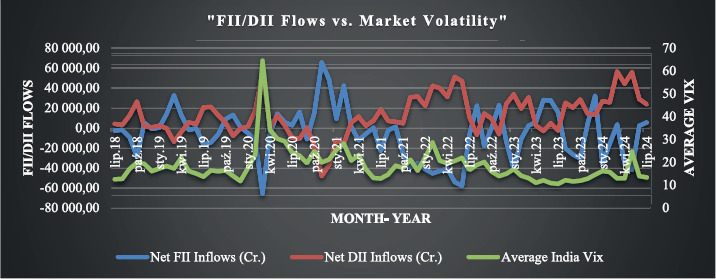
DII flows are counter-cyclical and tend to rise when FII outflows occur. The buffering effect was seen in March-April 2020, where DII inflows partially offset FII withdrawals, which contributed to a gradual decline in volatility. This underscores the stabilizing role of DIIs during market stress. Their sustained inflows since 2022, along with relatively stable or declining volatility, further underscores this contribution. Volatility also has a seasonal and cyclical nature with a tendency to peak at significant economic events such as geopolitical tensions and inflationary pressures during mid-2022. Divergent FII and DII flows increase volatility, whereas convergent flows have the opposite effect and tend to stabilize the market. To sum up, EDA reveals that sharp FII flows are the main driver of Indian market volatility, whereas DII investments serve to stabilize it.
Institutional Investment Behavior: Pandemic vs. Post-Pandemic
Net flow of FIIs and DIIs during pandemic period and post – pandemic period is shown in Table 1 where FIIs registered average monthly net outflows of ₹4,491.47 crore during the pandemic phase, demonstrating risk aversion and global uncertainty. In contrast, DIIs behaved counter-cyclically with average net inflows of ₹8,154.36 crore, balancing the market by taking up the supply generated due to FII exits.
Table 1
Pandemic vs. Post-Pandemic
Market volatility, as indicated by the India VIX, averaged 21.19%, and the Nifty 50 index oscillated around 11,315.92, reflecting a time of market tension. In the post-pandemic recovery phase, this trend reversed. FIIs came back strongly, recording average monthly net inflows of ₹14,514.18 crore, while DIIs recorded net outflows averaging ₹9,330.81 crore per month, perhaps taking profits or redeploying assets as market sentiment improved. Interestingly, volatility in the market climbed to 24.82%, even with the return of FII inflows, indicating doubt over inflation, global monetary tightening, or geopolitical concerns during the recovery phase. The average index level of the Nifty 50 increased to 12,271.50, indicating modest market recovery.
The relationship between volatility and institutional flows also shifted significantly over the two periods. The FII-VIX correlation decreased from -0.75 during the pandemic (strong inverse relationship) to -0.21 post-pandemic, suggesting that FII flows were more responsive to volatility during the crisis but less so during the recovery. For DIIs, the positive relationship with VIX decreased from 0.71 to 0.40, suggesting that their stabilizing behavior continued but was weaker. FIIs have the tendency to act pro-cyclically, exiting during periods of high volatility and re-entering in recovery phases, whereas DIIs tend to act counter-cyclically, providing market support during times of distress and trimming exposure as markets recover. These changes reflect the distinct role that each investor class plays in influencing market dynamics at times of crisis and recovery.
3.2 Stationarity and Model Diagnostics
The results of the Augmented Dickey-Fuller (ADF) test indicate strong confirmation that data are stationary. The ADF statistic at -4.5119 with a p-value of 0.00019 is significant at the 1%, 5%, and 10% levels (critical values: -3.5246, -2.9026, and -2.5887, respectively). The null hypothesis of non - stationarity is, therefore, rejected as it establishes a constant mean and variance across time.
3.3 Volatility Modeling using GARCH and EGARCH
Indian stock market volatility dynamics were modeled using a GARCH (1,1) model with VIX, FII flows, and DII flows as the main determinants. The results in Table 2 capture the dominant trends in market volatility. The significantly positive constant term ω depicts the underlying baseline volatility reflected in the VIX that operates in the market, regardless of the specific event-related institutional flows. The significant ARCH term is α = 0.5370, showing strong and immediate effects of past VIX shocks, with evidence of volatility clustering; a sudden FII outflow or inflow that triggers VIX spikes is likely followed by continued high VIX levels.
Table 2
Volatility Analysis
| Parameter | Coefficient | Standard Error | t- statistic | p- value | Significance |
|---|---|---|---|---|---|
| Omega(ω) | 0.0244 | 0.008886 | 2.747 | 0.006 | Significant |
| Alpha (α) | 0.5370 | 0.1939 | 2.768 | 0.057 | Significant |
| Beta (β) | 0.2100 | 0.1110 | 1.891 | 0.059 | Significant |
The borderline significant GARCH term is β = 0.2100, indicating moderate VIX persistence, suggesting that the impact of past VIX levels and, consequently, the impact of institutional activity fades relatively quickly. Critically, if the sum of α and β is less than one, then it indicates mean reversion. Although the β parameter is only borderline significant (p = 0.059), borderline persistence estimates are common in monthly volatility series, especially during structurally volatile periods such as the post COVID phase. Previous studies have documented that the maximum-likelihood standard errors in GARCH models may be conservative under non-normality and, therefore, borderline p-values are not a surprise. Because alternative models of this study specifically EGARCH and TGARCH also show a similar pattern of persistence, this inference of moderate volatility persistence thus remains robust, even without bootstrapped standard errors. Extreme VIX levels are normally caused by the activities of FII or DII and hence are transitory in nature, reverting to the baseline (ω), which would imply that long-term investment strategies are less prone to these fluctuations in short-term volatilities.
While the regular GARCH model does not account for asymmetric volatility effects, EGARCH (1,1) is especially formulated to do so – where negative shocks affect market volatility in a different manner compared to positive shocks. In this regard results shown in Table 3 where institutional flows like those from FIIs and DIIs display an imbalance of influence on the India VIX. The large ARCH coefficient (α = 1.3925) identifies that historical shocks in the form of abrupt VIX changes – have a powerful impact on current volatility, affirming the occurrence of volatility clustering.
Table 3
Asymmetric effect of Institutional
| Parameter | Coefficient | Standard Error | t- value | p - value | Significance |
|---|---|---|---|---|---|
| Omega(ω) | 11.7303 | 2.596 | 4.519 | 6.200 × | Significant |
| Alpha (α) | 1.3925 | 0.313 | 4.083 | 4.455 × | Significant |
| Beta (β) | 0.0638 | 0.211 | 0.302 | 0.763 | Insignificant |
Most significant, the model indicates a high degree of asymmetry: FII outflows create disproportionately more massive spikes in volatility than inflows have the ability to smooth out. This captures the so-called “leverage effect,” wherein bad news or selling provokes a sharper response from the market than good news. This is especially so in the Indian context, where mass FII selling can induce supply shocks and serve as an indicator of weakening sentiment, resulting in spikes in volatility. On the other hand, FII buying pressure is taken up more seamlessly, and therefore, inflows do not have an equivalent decrease in VIX. The GARCH component (β = 0.2100), although just bordering on statistical significance, reflects modest persistence of volatility. Nonetheless, DII action – necessarily contrarian in nature – is stabilizing in its effects. By acting in times of FII selling, DIIs keep the depth and duration of volatility in check, even though they do not lower it substantially. For investors, this asymmetric volatility implies that unfavorable shocks – most notably those attached to FII selling – have to be eyed closely since they can result in sudden and inflated market movements. In contrast, DII flows provide a buffering effect, ensuring that they become pivotal to marketplace resilience during agitated periods.
3.4 Liquidity and Volatility Interaction
Liquidity, usually measured by trading volume, captures the ease of trading without affecting prices substantially. This section explores how trading volume interacts with institutional flows – both FII and DII – and market volatility, as measured by the India VIX.
A high positive correlation (0.6383) between trading volume and India VIX is a sign that increased trading volume occurs when market volatility is present. This shows that uncertainty results in increased participation by investors because of speculative flows, portfolio balancing, and risk aversion plays. Although an increase in trading volume can promote liquidity, it also reflects market stress, mostly accentuating volatility – especially among emerging markets such as India. The poor positive correlation (0.1893) between trading volume and FII inflows suggests that FIIs, while adding to market depth, do not influence short-term trading activity directly. Their generally long-term focus results in their effect on liquidity being more significant in periods of stability than in times of volatility. On the other hand, the negative correlation (-0.2977) between DII inflows and trading volume emphasizes the counter-cyclical and stabilizing nature of domestic investors. DIIs increase their presence in the market during low-volume periods – usually when volatility is increasing – and decrease activity when trading increases, so as not to further disturb the market. This reflects their contribution to liquidity support during quiet times and dampening excesses during turmoil.
Overall, the interplay indicates a subtle interaction: although volatility translates into higher trading activity, institutional flows are not all equivalent in their contributions. FIIs increase liquidity in quieter times, while DIIs play a stabilizing role, strategically offsetting volatile patterns and supporting market stability.
3.5 Dynamic Interactions using VAR Model
The VAR model was estimated using monthly data from July 2018 to July 2024 for FII Inflows, DII Inflows, India VIX, and Market Volume. The optimal lag length was determined using the AIC/BIC criteria, and the model was found to be stable, with all roots lying inside the unit circle. Diagnostic tests showed no significant autocorrelation (p = 0.113), indicating that the model is correctly specified and the residuals are uncorrelated. The stability test confirmed the model’s reliability, ensuring that shocks will not cause explosive behavior. However, the residuals deviated significantly from normality (p < 2.2e-16), suggesting that the standard errors might be biased. Non-normality of residuals does not weaken the VAR estimates because, according to Lütkepohl (2005), the OLS estimation of VAR coefficients is consistent even under deviations from normality. Moreover, impulse responses and variance decompositions still provide a valid structural insight into the analyzed model when it is stable. Financial time-series data are often not normally distributed, as they are plagued by fat tails and volatility clustering; thus, the non-normal errors are not damaging for inference as long as autocorrelation and stability conditions are satisfied, which is the case here. Despite this, the Granger causality results remained robust. These findings suggest that while the model is reliable for dynamic analysis, using more robust estimation techniques, like bootstrapping, could help refine the results and improve precision.
Granger Causality Analysis
Pairwise Granger causality tests were carried out to test if previous levels of FII flows, DII flows, market volatility (India VIX), and trading volume can statistically forecast movements in each other. Although not establishing true causality, the results shed light on the strategic autonomy of institutional investors and their response to market conditions.
The analysis reveals that FII flows do not Granger-cause DII flows, VIX, or trading volume, as all p-values (FII→DII: 0.673, FII→VIX: 0.344, FII→ Volume: 0.763) are larger than the 5% significance value. This indicates that FIIs seem to move autonomously, possibly based on overseas drivers like interest rates, geopolitical tensions, and currency shifts, rather than domestic market dynamics. Likewise, DII flows do not have a strong predictive power for FII flows, VIX, or volume (DII→FII: 0.290, DII→VIX: 0.833, DII→ Volume: 0.658). This supports the notion that DIIs move independently and are more driven by long-term fundamentals. Their interventions seem counter-cyclical, focused on market stabilization rather than trend initiation. Granger tests for India VIX predicting flows and volume (VIX→FII: 0.550, VIX→DII: 0.167, VIX→ Volume: 0.693) also did not provide any statistically significant findings. This suggests that volatility, as captured by VIX, does not systematically drive institutional action or trading in a predictive sense. One exception is the Volume→ DII relationship with a p-value of 0.078 and marginal significance at the 10% level. This can be interpreted that DIIs would react to more trading activity as an opportunity to stabilize markets or pick up on undervalued assets during times of high volumes. This also fits their image as liquidity providers during volatile times. The other reverse relationships, i.e., Volume→ FII (0.491) and Volume→ VIX (0.124), were insignificant, indicating that trading volume per se does not forecast foreign investor actions or future volatility.
Empirical evidence from Granger causality tests shows that there are weak predictive links between market volatility, institutional flows, and liquidity. FIIs and DIIs move independently to a great extent, reacting to current market conditions and not to their past movements. A marginally significant relationship from trading volume to DII flows implies that domestic investors can fill the gap during increased activity, supporting their stabilizing function. For regulators such as SEBI and RBI, the absence of high lag-based predictability suggests limited systemic risk of herding and argues in favor of emphasis on real-time monitoring rather than predictive modeling. For fund managers and investors, the results warn against dependence on past data; instead, focus must be on recent macroeconomic indicators and sentiment data.
While lag-based projections are limited, Impulse Response and FEVD analyses indicate that shocks in FII inflows lower volatility, while DII inflows raise liquidity – highlighting the significance of institutional flows in influencing near-term market action and informing strategies based on timely data and structural insight.
Response of India VIX to a Shock in Net FII Inflows
The impulse response function (IRF) in Figure 2 embodies the reaction of India VIX to a one-standard deviation shock in Net FII Inflows. India VIX reacts negatively in the short run, suggesting that an increase in FII inflows decreases market volatility.
Figure 2
Response of India VIX to a Shock in Net FII Inflows
The solid black line represents the estimated impulse response of India VIX to a shock in Net FII inflows over the forecast horizon. The red dashed lines indicate the 95% bootstrap confidence intervals (100 bootstrap runs), while the horizontal red line denotes the zero-response benchmark. A negative response indicates a decline in market volatility following an increase in FII inflows
Source: authors calculations.
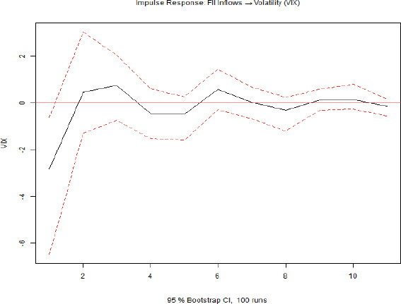
The fact that it is negative indicates that foreign institutional investor inflows are viewed as an indicator of market confidence and decrease perceived risk. The impact, although initially significant, diminishes over time and converges to zero on a medium-term horizon (around 4-6 months), suggesting that the impact of FII inflows on volatility is temporary but considerable in the short term.
Response of Market Volume to a Shock in Net DII Inflows
The IRF in Figure 3 shows the response of Market Volume to a one-standard deviation shock in Net DII Inflows. The response is positive and long-lasting, suggesting that domestic institutional investor activity induces market participation and liquidity.
Figure 3
Response of Market Volume to a Shock in Net DII Inflows
The solid black line represents the estimated impulse response of Net DII Inflows to a one-standard-deviation shock in market trading volume over the forecast horizon. The red dashed lines indicate the 95% bootstrap confidence intervals obtained from 100 bootstrap replications, while the horizontal red line represents the zero-response benchmark. Positive values indicate an increase in DII inflows following a rise in market trading volume.
Source: authors calculations.
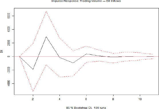
The impact lasts for a few months before it decays, indicating the liquidity-promoting function of DIIs in the Indian stock market. This corroborates the hypothesis that DIIs, while more cautious than FIIs, play a significant role in market depth and flow of transactions.
Forecast Error Variance Decomposition (FEVD)
The FEVD results, as shown in Figure 4 provide a breakdown of the degree to which each endogenous variable explains the forecast error variance of India VIX over time. In the early months, the variation in India VIX is dominated by its own shocks, indicating a strong autoregressive element in market volatility. But as the forecast horizon lengthens, the importance of Net FII Inflows starts featuring more prominently, explaining a large part of VIX’s variance. This is also in accordance with impulse response analysis that identified the strong impact of foreign capital flows on volatility.
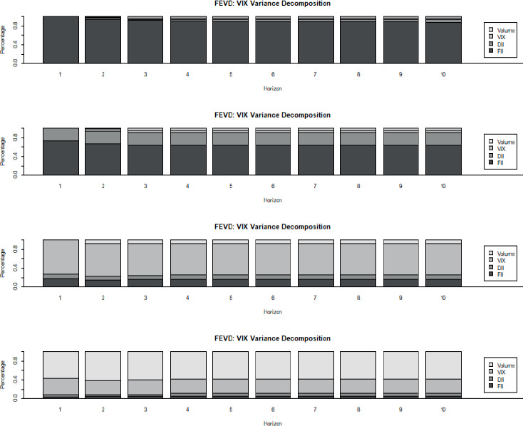
Conversely, the role of Net DII Inflows and Market Volume in explaining the forecast variance of VIX is comparatively small over the period, reflecting their marginal contribution to volatility driving. Overall, the FEVD analysis supports the interpretation that FII-related shocks are an important driver of movements in India VIX, highlighting the intimate connection between foreign investor activity and market sentiment in the Indian equity universe.
4.0 Conclusion
The paper examines the complex inter-dynamics between institutional investors – viz., Foreign Institutional Investors (FIIs) and Domestic Institutional Investors (DIIs) – and a couple of other key market parameters including volatility, gauged through the India VIX, and liquidity, indicated by volume of trading, in the Indian capital market. Exploratory analysis, along with pandemic as well as post-pandemic breakdown, presents the fact that FII withdrawal is strongly related to sharp volatilities spurts, mirroring volatility clustering. Formal stationarity tests validated the suitability of the selected variables for time-series modeling. The GARCH analysis confirmed persistent volatility in the market, underscoring that shocks have long-lasting effects. Notably, EGARCH results revealed a significant asymmetric volatility effect, whereby negative shocks often associated with FII selling – trigger disproportionately larger increases in volatility compared to positive shocks. This “leverage effect” proves the market’s increased vulnerability to bad news, confirming the systemic relevance of foreign capital flows.
Liquidity dynamics also explained the differentiated function of institutional investors. High positive correlation between India VIX and trading volume shows that volatility drives trading activity, evidencing reactive behavior among the market participants. FIIs, though adding to market depth, displayed a poor correlation with trading volume, indicating a more strategic and long-horizon impact. DIIs, on the other hand, played a counter-cyclical stabilizing role, as their flows negatively correlated with market volume, indicating that domestic institutions ramp up participation in times of market decline and moderate activity in times of overheating, thereby ensuring market equilibrium. The addition of Granger causality tests provides a further layer of sophistication. The findings indicate weak predictive relationships between institutional flows, volatility, and liquidity, so that FIIs and DIIs move relatively in tandem and react more to contemporaneous factors than lagged interdependencies. Nevertheless, a marginal predictive signal from trading volume to DII flows indicates that domestic institutions do respond to increased market activity, supporting their stabilizing role. The VAR model, complemented with Impulse Response Functions (IRFs) and Forecast Error Variance Decomposition (FEVD), offers more structural insights. Though Granger causality indicates restricted lag-based predictability, IRF estimates uncover that shocks to FII inflows are found to lower market volatility, and shocks to DII inflows increase market liquidity. The FEVD results also verify that in the long run, an increasing proportion of volatility (India VIX) is accounted for by innovation in FII flows, making foreign capital an important driver of sentiment in the market. By contrast, the DIIs’ and trading volume’s contribution to volatility variance is still small, supporting the notion that DIIs play a stabilizing rather than a destabilizing role.
This multi-method study re-affirms that FIIs have a strong and asymmetric impact on market volatility, especially during phases of negative sentiment, while DIIs act as counter-cyclical stabilizers in the Indian stock market. Results of EGARCH modeling, VAR analysis, Impulse Response Functions (IRFs), and Forecast Error Variance Decomposition (FEVD) together affirm that even if institutional flows are not shown to have statistically significant lag-based predictability, their real-time and structural effect is quite high.
At a policy level, these findings point to the imperative for market regulators like SEBI to vigilantly observe FII activity, particularly during times of high volatility, as FII outflows tend to disproportionately magnify market uncertainty. Strengthening circuit breakers, better risk-based margining, or using macroprudential instruments during sudden-withdrawal capital outflows would help reduce system shocks.
To fund managers and retail investors, the analysis offers something tangible: timing and trend in institutional flows – and especially FII exits – need to be understood as precursors to possible spiking volatility. On the contrary, rising participation by DIIs during declines should be interpreted as a sign of stabilization, as a tactical long-term entry signal. As foreign capital flows shape domestic markets in the future too, diversification, volatility guarding strategies, and understanding institutional behaviour become essential components of portfolio management. This research adds not only to scholarly writing on capital market dynamics but also to practical applicability for regulatory control and investment planning in a more interconnected global financial system.
Limitations and Future Scope
While this research emphasizes the manner in which FIIs enhance short-term volatility and DIIs have a stabilizing influence, certain limitations and subtleties need to be acknowledged. The absence of lag effects in Granger tests is at odds with pronounced real-time effects in VAR and IRF, highlighting that institutional flows have an immediate impact on markets, not with a time lag. FIIs lead to panic in the short term (according to EGARCH), but dampen volatility in the long run (as evidenced by FEVD). Methodologically, using daily data may not capture rapid market response, and linear models could miss non-linear behavior. Subsequent research based on high-frequency data with sophisticated models may provide greater insights into institutional market behavior. While these limits exist, our conclusions still provide useful value: they enable market regulators to recognize possible dangers, benefit investors by helping them make better choices, and add to our general knowledge about how institutional investors shape stock markets in developing economies such as India.